
This paper intends to introduce the Polynary (pa’-le-nair’-ee) approach to data analysis. Polynary is mathematically simple compared to conventional statistical methods. Polynary was developed from listening to how people describe collections of similar objects, characterize objects in a way that places them into different categories, and how they explain something by describing one thing in terms of something else. These things have parallels to quantitative methods commonly used by data analysts. The Polynary approach leads to a high-dimensional coordinate system rendered on a two-dimensional surface. And its analytic results are expressed in language (English). It aims to make data and the claims made from it more transparent to clients, decision makers, and broader audiences. The author welcomes your helpful comments at suppoort@polynary.com.
Table of Contents Page
Introduction………………………………………………………………………………………………………….…….1
How Polynary Strings Partition a Dimensional space ……………………………………………………….2
Unit-Cubes: Interpretive Context and Data Scaling……………………………..……………………………4
Transforming Rectangular Coordinates to Relative Coordinates…………………………………………5
Representing Relative Coordinates as a Polynary String……………………………….……………………6
Introduction to Polynary Graphs…………………………………………………………………………………....7
Illustrating the Polynary graphs for Addition and Subtraction…………………………….…… ………11
Interpretation of Graphs…………………………………………………………………………………………..…..12
Making Sense of Quantifying Adverbs……………………………………………………………………………..13
The Construction of Description…………………………………………………………………………………..…14
The Parsing Problem—Why these Descriptions?……………………………………………………….……….15
The Method of Natural Clusters………………………………………………………………………………………16
Summary Remarks and Applications……………………………………………………………………….…..….17
Converting a set of M relative coordinates into a polynary string……………………………… ..……19
Introduction
Few claim they can imagine more than 3-dimensions. Try as we may, we can’t draw another axis perpendicular to the first three. Seeing and reasoning in high dimensional spaces seems foreclosed to us.
But is it? I can, for example, describe Wisconsin’s April weather as: “somewhat cool, quite rainy, moderately humid, and very cloudy”. Somehow, descriptions that string together a set of adverb-adjective pairs makes sense to people. And notice this description is 4-dimensional--something we just suggested we couldn’t imagine!
What gives? The parallel between math and language is direct. In language we use nouns (or adjectives) to refer to dimensions, and we replace numbers with adverbs to connote the degree, extent, or amount of something. Yet somehow language isn’t bound to the low-dimensional world of Descartes. The real world is truly complex. And once we start paying attention, we see that people think and talk about high-dimensional quantitative ideas every day; we just don’t think of it as geometry or math.
Marvin Minsky, a founding father of AI, long ago pointed out that the way we represent information changes everything. It changes how we think, what it is good for, how we process it, and the form of the answers it spits out. Brain and school math feel different because they are different computational systems. One uses words, the other numbers. We can imagine more than three quantitative dimensions. It’s just that Cartesian boxes can’t match the higher dimensional realm of minds and the language answers they spit out.
Can observations about how we describe things teach us about how to see high-dimensional data spaces?We think so. This is a critical bridge because geometrically the information in data is in the patterns they form, and our eyes are the best pattern detectors around! To reach this goal, we must reconsider the way we represent information to parallel how we describe quantitative ideas in language. We call this new approach Polynary
How Polynary Strings Partition a Dimensional Space
Let’s begin by talking about how a set of an object’s quantitative features become represented by a single polynary string. You can think of it as a kind of generalization of binary. We will cover the technical details later. For now, it is easiest to develop the approach intuitively through the Cartesian geometry we already know.
In the 2-D Cartesian plane we traditionally treat an object as a point determined by two numbers (x,y). We can divide this plane into graph paper like cells, as in Figure 1. If we divide each dimension in half, we get 4 cells; divided in thirds we get 9 cells, and so on. We can informally describe these cells in language by citing a noun-adverb combination for each dimension.
Figure 1. The Graph Paper partitions of the Cartesian Unit-cube.
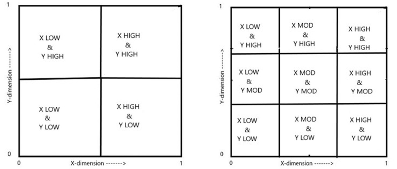
Every point will fall into one of these cells. Unfortunately, this approach falls apart after three dimensions. But there are other ways of dividing space. The first division in Polynary (schematically show in Figure 2) divides the (x,y) Cartesian plane into 3 cells . Each cell is called a polynary basin because every point will fall into one of these geometric regions. In the left panel we denote each basin by a single letter (symbol), either X, Y, or 0, as the first letter of its Polynary string.
Figure 2. The first two Polynary partitions of the Cartesian Unit-cube.

We will later come to connote these basin regions through descriptions as, for examples, in basin 00, X and Y are both extremely to quite low; in 0X, X is moderate and Y very to somewhat low; in X0, X is somewhat high and Y very to barely low; in X, X is extremely high and Y is low; and in X, X is somewhat to extremely high, Y quite moderate to barely high. All the objects (data points) falling into a given basin share a common description. Within the context of a dimensional frame, a description connotes the location, shape, and size of a geometric sub-region of space. This is what quantitative descriptions do.

The 27 basins at the 3rd partition of the plane become denoted by strings 3 symbols long.
Basin size shrinks with each additional letter. As this happens, every (x,y) point becomes more closely approximated by a Polynary string. This convergence happens very quickly.
We can effectively represent and replace (x,y) pairs of numbers to any degree of precision we desire though a single Polynary string of sufficient length.
As the string becomes longer, the corresponding basin descriptions become more specific.
The way Polynary divides space is unlike the graph paper grids we learned in school. But we can apply the logic of this sequential division process to any number of dimensions in a completely analogous way. Importantly, there is an extremely simple algorithm that converts an N-dimensional set of numbers into its corresponding Polynary string. We won’t need in future to concern ourselves with the rather odd way Polynary partitions space; the only notions we need to carry forward involve certain geometric reasoning:
1) A Polynary string is a unique address to a contiguous chunk of N-dimensional space, the spelling of this address contains information about its location and size within this space.
2) The longer the string, the smaller the chunk.
3) Each N-dimensional chunk has from N to 2N identifiable neighboring chunks.
4) The collection of chunks accounts for the entire space.
These geometric properties allow us to extend spatial reasoning into high-dimensional spaces. The dimensionality of the chunk and its size makes no difference; a chunk of space is just a chunk of space. All the points in the same basin characterize objects that are similar and share a common description. This similarity increases as we increase the length of the string. And because the size of these regions become smaller as strings get longer, their corresponding descriptions become more specific.
Unit-Cubes: Interpretive Context and Data Scaling
Whenever we measure multiple properties of an object, the numbers along each dimension generally come from different kinds of rulers. A direct comparison of values between them are meaningless. We can always align the directional sense of each dimension so that smaller values mean less, and larger values mean more, based on how we choose to name the dimension.
Of course, we give numbers meaning when we devise standardized rulers. It makes sense to say that someone is 72 inches tall and weighs 220 pounds. But these numbers are still arbitrary. Equivalently, I could have said 1.83 meters and 100 kilograms. We need a way to assign numbers to concepts that is independent of our choice of ruler, and subsequently, to give contextual meaning to adverbs.
Something known as conceptual variables achieves this. We understand the question “On a 0 to 100 scale how happy are you?” It is the relative position along this scale that conveys the meaning of your answer. The meaning of a number is set by its location relative to scale endpoints as defined by the data’s minimum and maximum values. It no longer matters whether you used inches and pounds or meters and kilograms; their numeric values become the same. The contextual meaning of a number comes from its relative position, where larger values mean ‘more’ of something and smaller numbers mean ‘less’.
Conceptual variables have a crucial simplifying benefit, they offload the need to track specific units of measure. They are unit-less quantities. Each dimension is scaled to a value between zero and one; creating something known geometrically as an N-dimensional unit-cube.
We can transform the data to a unit-cube in other ways. For example, we can replace the values along each dimension by their rank values. The lowest rank is assigned to zero, and the highest rank a value of one. Tied values are given the same rank. This transformation preserves the order of the values along a dimension while sacrificing the distance between consecutive points. Here, the meaning of a number comes from its relative rank. Again, there are no units of measure.
One advantage of ranks is that the values of different dimensions are comparable. For instance, being at the 50th percentile of Agreeableness and Conscientiousness means you are in the middle of both of these dimensions relative to the other people in the sample. This is different from scale-relative where all you can say is that both are at the midpoints of their individual scales.
People are familiar with scale-relative and rank-relative interpretations. For instance, your cholesterol might be “very high” in the context of medical standards, but only “somewhat high” relative to other people in your age group. What we say or hear depends on the context we give it; sometimes we have to ask for clarification.
But the result of the scaling choice is the same. We have an N-dimensional unit-cube where the values of each dimension are between zero and one and where larger values indicate more of something. Adverbs like ‘very’ and ‘somewhat’ only acquire meaning through the context of scale endpoints. This is the reason we work through unit-cubes and showed the partitioning in the Figures above as squares.While the unit-cube framework is simpler than a generalized rectangular box, no information is lost. The two are mathematically equivalent.
Transforming Rectangular Coordinates to Relative Coordinates
In the N-dimensional unit-cube framework, an object is a point identified through an ordered set of rectangular coordinates we denote as { z(1), z(2), …, z(N) }. Each value reflects how ‘much’ something ‘is’ in absolute terms. We want to characterize this information in relative terms.
The reason is that objects may have many dimensional properties, but it is rare in language to cite more than some combination of three dimensions when we describe them. A common and effective strategy is to only cite those features of an object that most stand out. This strategy efficiently draws distinctions between objects by citing the different ways they are notable. For instance, “Jane is very agreeable and quite conscientious, and Tom is very neurotic”. We understand in language that we all share the same set of personality traits, but what distinguishes us is the relative degree they animate who we are.
To transform absolute to relative coordinates, we need to create a slack variable; an overall composite measure of what this set of values ‘is not’. We need this because it may be that the most notable feature about an object is that none of the dimensional values stand out. This enables shorthand statements like “Mike has a wallflower personality” to mean his personality has no striking features. We begin this transformation by noting that the complement of each dimension is given by 1-z(n). Here, we define this slack variate, z(not-ness), as the geometric mean of these complements.
The value of z(not-ness), like the others, is always between zero and one; but its value sense runs opposite to the other z-values. That is, its value approaches 1 as all the formal z-values approach zero, and it approaches 0 as all the formal dimensions approach a value of 1. In adding z(not-ness) to the N formal dimensions, there are now (N+1) quantified concepts for each object.
The information we need from these (N+1) measures is their relative magnitude—and we can express this by turning them into a set of proportions. This is done simply by dividing each of the (N+1) measures by their sum. The resulting values are a set of proportions that express the relative degree an object’s features stand out in relation to the whole. We call these proportions relative coordinates to distinguish them from natural proportion data, but their properties are identical: Every number is non-negative and together they sum to one.
There is a unique one-to-one mapping between a point in an N-dimensional conceptual space which we denote as { z(1), z(2), …,z(N) } and its corresponding set of relative coordinates { p(1), p(2),…,p(N+1) }. The two sets of numbers are simply different representations of the same quantitative information—nothing lost, nothing gained. It is just a transformation of coordinates.
We make this move because a description of an object focuses on the relative degree its dimensional features stand out. With the added concept of ‘not-ness’ we can cover the situation where what is most notable is that none of the formal variable values stand out. This prevents getting painted into a logical corner. In effect, it adds the option of saying ‘neither’ to the question: “Do you want to get punched or kicked?” The introduction of the slack variable restores the sense of absolute values within the space of the unit-cube.
Representing Relative Coordinates as a Polynary String
The transformation from rectangular to relative coordinates still represents objects through sets of numbers. The critical difference is that an object’s relative coordinates can be ‘digitized’ into a single polynary string through a simple algorithm. Analytically, this string representation is like a generalization of binary. Instead of two symbols Polynary uses M symbols; one symbol for each of the M relative coordinates in the set. Binding the multiple aspects of an object into a single string makes sense because an object is the smallest logical unit of analysis. One object, one string.
In a previous section we showed the nature of how a unit-plane is sequentially sub-divided as we increased the length of the polynary string. Higher dimensional cubes become partitioned in an analogous way. As the Polynary strings becomes longer, the corresponding chunks of space they denote become smaller. In fact, the volume of these chunks (basins) rapidly converge to zero as their average volume becomes about M times smaller with each letter added to the string. We present the algorithm for transforming relative coordinates to a string as an endnote [i].
Through this algorithm we can represent an object’s set of relative coordinates to any degree of numeric precision desired. This means that no matter how little two objects quantitatively differ; their strings will have different spellings if their length is sufficiently long. For background, we point out that the successive values of G in the algorithm form a geometric series whose values only depend on M. This series ‘digitalizes’ relative coordinates into a string more efficiently than any other.
The previous sections provide a pretty detailed outline of the transformation from the numeric representation of objects to the representation as polynary strings. There is a mathematical equivalence between the two.
The rescaling of data from rectangular Cartesian space into the unit-cube puts the numbers coming from different rulers into a common conceptual framework of unit-free measures. This move is necessary, as described later, to give the adverbs their contextual meaning. The transformation of the set of conceptual rectangular coordinates into relative coordinates characterizes an object by the relative degree its dimensional features stand out. This mirrors how people distinguish objects by focusing on the way(s) that they are most notable. And finally, a polynary string binds these dimensional properties of an object into a single logical unit. This makes sense because people form generalizations and claims over objects not their individual measures. We can now explore some of the consequences.
Introduction to Polynary Graphs
One key benefit of representing data in the form of polynary strings is a coordinate system that allows us to visualize high dimensional spaces on a two-dimensional surface. For 2-D problems we will need a fractal based on a triangle—one for each different symbol we used for the Polynary strings. For 3-D we use a square fractal, for 4-D a pentagon, and so on.To begin, in Figure 2 we schematically showed how we sequentially partition a 2-dimensional plane. We reproduce this in Figure 4. This will allow us show how Polynary strings lay out on its corresponding fractal in Figures 5 and 6.
Figure 4. Schematic of the first two Polynary partitions of the Cartesian Unit-cube.


In the left panel of Figure 4, the first letter of the Polynary string divides the plane into 3 chunks—where X was relatively large, where Y was relatively large, and 0 where neither is relatively large.
In the Polynary graph on the left, we represent these three basins as circular rose-colored regions on the graph, each chunk labeled with its Polynary string.
To avoid confusion with letters, we sometimes use “▼” instead of “0” on these graphs to indicate jointly smaller values of x and y. This symbol will always point downward to remind us that this direction indicates the set of values are smaller.

In the right panel of Figure 4 we partition the plane for the second time, breaking each of the three larger chunks into three smaller regions yielding a total of 9 basins.
In the Polynary graph on the left we represent these divisions by dividing each larger circle into three smaller circles. We show the strings associated with each circle using two-symbols strings.
Notice that the layout of these strings respects the same directional sense found on the earlier graph. XX is found in the upper-right corner, YY the upper-left corner, and 00 is at the bottom.
With the graph above we can start to see the fractal nature of the coordinate system and some of its properties. Notice, for example, the ordering of Polynary strings along the outer edges of the graph. The basins from 00…XX and from 00…YY appear in ‘binary’ order. And the basins YY…XX along the top show a ‘binary’ exchange in the values of x and y.
Let’s continue this division process one more time, showing the partitions and their graph.
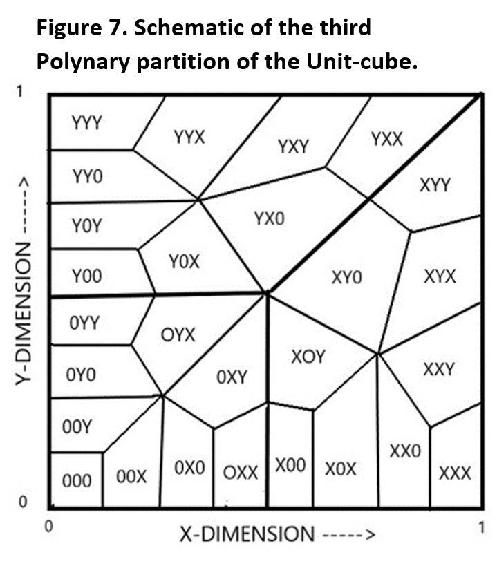
The third Polynary partition divides the prior regions again, giving a total of 27 basins. A unique string three symbols long denotes each of these basins.
We see basin size shrinks with string length.As this happens, every (x,y) point becomes more closely approximated by a Polynary string.This convergence happens very quickly.
Analytically, the Polynary string representation of relative coordinates can represent (x,y) pairs of numbers to any desired degree of precision though a long enough string.
It is clear the points in the plane become grouped into basins. Objects that fall into the same basin are alike in the relative way the values of their dimensional features stand out. While how Polynary partitions space may seem odd at first, the divisions better account for how we flexibly use partial descriptions to characterize high-dimensional objects. We elaborate on this observation and put it to good use later.
The basins of Figure 7 organized and arrayed on the fractal structure are shown in Figure 8.

This fractal structure provides a simple, coherent, visual organization to polynary strings. The layout respects the same directional ordering indicated by the central letters at all size scales. As a coordinate system we can identify the location of any string from its spelling and determine its spelling from any location. For example, the location to XY0 is found in three directional steps from the graph’s center. First move in the X-direction, then the Y-direction, and then in the ▼direction.
We can repeat this division logic for as long as we like; each previous circle becomes three smaller circles. And as we do this the space becomes divided into ever smaller chunks. In the limit every real point in the plane has a unique polynary string with a volume of zero. But this is unimportant; the information in data is in the patterns they contain. And these features are emergent properties that exist over regions of space that are much larger than individual points.
The ideas developed here using the 2-D plane can be generalized. They apply to higher dimensional spaces in directly analogous ways. For example, the 5-dimensional graph of Figure 9 uses six symbols; one for each formal dimension, and a ▼ symbol to indicate ‘lower values’ across the 5 formal dimensions. This results in a fractal based on a hexagon like that shown below.

Note that this graph divides 5-D space into 36 basins through Polynary strings two-letters long.
Strings just one letter longer creates 216 basins, drawing distinctions that cover, on average, less than a half of one percent of the 5-D space.
Using the same ordination principle, we can locate any Polynary string from its ‘spelling’, and we can determine its ‘spelling’ from its location. For instance, we show the basin FA is located by the path of two lines from the center of the graph.
We now have all the essentials of a coherent high-dimensional coordinate system.
Illustrating the Polynary graphs for Addition and Subtraction
Let’s apply this coordinate system to the simplest mathematical functions—addition=x + y, and subtraction= x - y. The X and Y values define the coordinate system and the value of the sum is indicated by the height (and redundantly, the color) of the bar. What does the visual interpretation of these graphs tell you?

The lowest sum occurs at the bottom of the graph where x and y are at their smallest. The highest sums occur at the top-center of the graph where both x andy are at their largest.
Notice the trend of increasing sums as you go from the bottom to the top of the graph. And notice the right-left symmetry across the middle of the graph. It shows that x and y are equally important to the value of the sum.
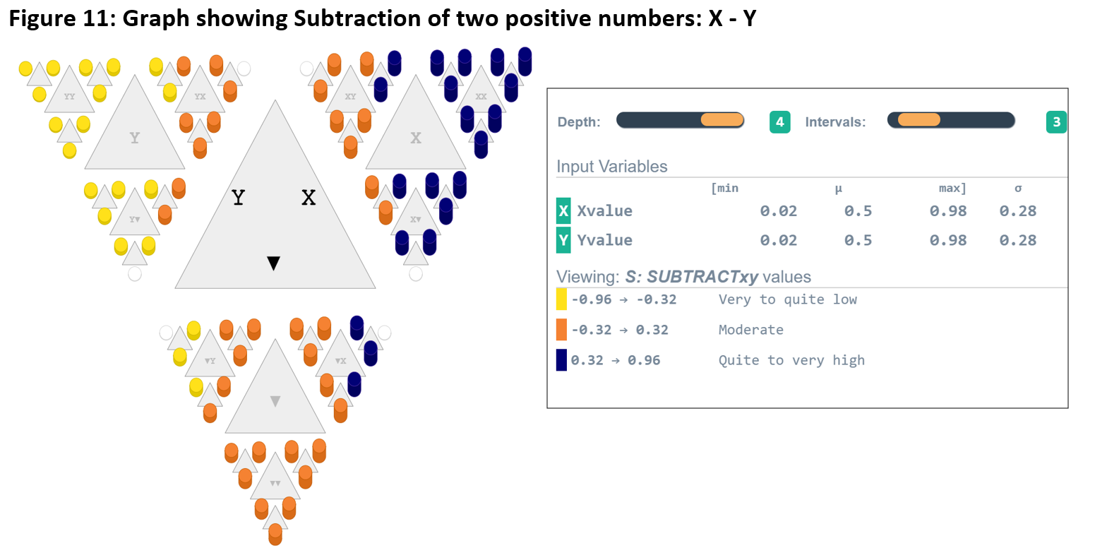
When x an y are positive values, the result of Subtraction is largest when x is large and y is small—in the X-corner of the graph. And the value of a Subtraction is smallest when x is small and y is large—found in the y-corner of the graph. Notice that the orange basins representing near zero values lay along a central line through the middle of the graph. This is where the values for x and y are nearly equal.
While this is a simple example, we can apply this technique to understand the behavior of any high-dimensional function. This exposes otherwise incomprehensible functions to the visual system for scrutiny—making their behavior easy for anyone to grasp.
The examples in Figures 10 and 11 show that that different relationships reveal different patterns on the coordinate system. And their informal visual interpretation comes with a little experience; we can see various contingencies of inputs where the outcomes are high, low, and in between.
Summary Remarks and Applications
We have outlined the nuts and bolts of the Polynary framework. The math behind it is simple but it changes how we represent information, and how we see and approach quantitative problems. This change in thinking takes a little time.
Paying attention to how people describe things suggested a change from rectangular coordinates to relative coordinates. Many math problems are simpler to solve by a change of coordinates, for instance cylindrical and polar coordinates, so there is nothing new here. Relative coordinates reflect what and to what degree the dimensional values of an object stand out.
This mirrors how descriptions can draw distinctions between objects by citing the different features that make them notable. Importantly, a polynary string binds the properties of an object into a single conceptual entity. The ‘spelling’ of this string reflects the value of its’ relative coordinates; and this string can represent them to any degree of precision desired.
We showed how polynary divides a unit-plane. These kinds of divisions occur in a parallel way in all N-dimensional unit-cubes. We did this to build a geometric interpretation of polynary strings. A polynary string represents a contiguous chunk of N-dimensional space. And each chunk has from N to 2N other chunks adjacent to it. For any given string, the polynary strings of these neighbors can be determined through a simple algorithm.
Through this geometric understanding we can easily extend spatial reasoning into higher dimensional spaces. To facilitate high-dimensional thinking we don’t have to know what these chunks look like, only that chunks are next-to other chunks. A polynary string uniquely labels each chunk. The average volume of this chunk becomes about (N+1) times smaller with each letter we add to the string. And the spelling of the string points to the location of its chunk within the N-dimensional unit cube.
An important benefit to the polynary string representation is that high dimensional objects can be plotted on onto a coordinate system rendered on a two-dimensional surface. This allows people to directly see and share the empirical data. This extends spatial reasoning into high dimensional spaces.
Notes
[i] To convert a set of M relative coordinates into a polynary string let:
P(m), m=1,2,..,M represent a set of M relative coordinates in a fixed order.
S(m), m=1,2,..,M be a set of M unique symbols representing the corresponding coordinates.
G initially be a number equal to 1/M.
B be a constant equal to the number (M-1)/M.
K= the total length of the Polynary string desired.
PolynaryString[k], k=1,2,…,K represent the K symbols in the resulting Polynary string.
k is initially 0; we use it to count how many times we go through the following repeat loop.
Repeat [Repeat the following instructions K times.]
k=k+1. [Index to the current symbol position in the string.]
Find J = subscript of the largest coordinate P(m) in the current list of M coordinate values.
(Resolve ties by selecting the lowest value of J; the first largest in the list.)
PolynaryString(k) = S(J) [The kth symbol of the Polynary string is S(J).]
P(J) = P(J) – G [Reduce the value of P(J) by subtracting the current value of G from it.]
G = G * B [Update the value of G by multiplying its current value by B.]
Until (k=K) [Terminate repeat loop when k equals desired string length.]
© PolynaryThink, LLC 2019 All Rights Reserved